11. 3D Data Fusion

Multi-modal fusion, ICP registration, TSDF, rolling buffer, SVD pose estimation

Contents

1. Overview and Motivation 2. 3D Data Types and Representations 3. LiDAR vs. RGB-D 4. Three-Stage Fusion Pipeline 5. Stage 1: Unifying Data Format 6. Stage 2: Unifying Coordinate Space 7. Stage 3: Fusing into a Unified Model 8. KinectFusion Limitations 9. Solution: Rolling Buffer 10. Drift and Geometry Melting 11. Solution A: Chained TSDF Boxes 12. Solution B: Plane-Based Drift Correction 13. SVD-Based Pose Estimation Interactive: SVD Walkthrough Flashcards

1. Overview and Motivation

This module addresses two major topics in 3D computer vision. First, fusing data from different modalities — combining point clouds (LiDAR), depth maps, and RGB images into a single coherent 3D model. Second, overcoming KinectFusion limitations — solving the practical constraints of real-time TSDF-based 3D reconstruction: limited volume size, drift, and geometry melting.

Why multi-modal fusion matters

No single 3D sensor captures a perfect scene. LiDAR provides accurate, large-scale point clouds but with many holes from occlusions. RGB-D cameras give dense, colorful local reconstructions but are noisy with limited range. Combining them yields a model that is both globally accurate (from LiDAR) and locally dense (from Kinect).

2. 3D Data Types and Representations

Sensor Modalities

Sensor Type	Output Data	Dimensionality	Scale
LiDAR	Point clouds $(x, y, z)$ with optional color/intensity	3D	Global, large-scale
RGB camera	2D color image	2D	Depends on lens
ToF camera	Depth maps	2.5D	Local, limited range
Structured light (Kinect)	Depth + RGB maps	2.5D	Local, ~0.5–4.5 m

3D Representation Formats

Representation	Pros	Cons
Voxel grid	Regular structure; easy to process with 3D CNNs	Memory-intensive $O(n^3)$; fixed resolution
Octree grid	Memory-efficient; only subdivides where detail exists	More complex data structure
Mesh	Compact surface; good for rendering	Hard to update incrementally
Point cloud	Raw, lossless; no discretization	Unstructured; noisy; redundancy
Depth maps + poses	Compact storage; easy to capture	Only 2.5D; requires pose information

Why fusion is non-trivial

The core challenges when fusing data from different sensors:

Different data formats: LiDAR produces 3D point clouds; Kinect produces 2.5D depth + RGB images.
Different data densities: LiDAR is sparse; Kinect is dense.
Different noise characteristics: LiDAR has sparse gaps; Kinect has quantization artifacts.
Unrelated coordinate systems: Each sensor has its own reference frame.
Incompatible intrinsic parameters: LiDAR has no focal length in the traditional sense.

3. LiDAR vs. RGB-D Sensors

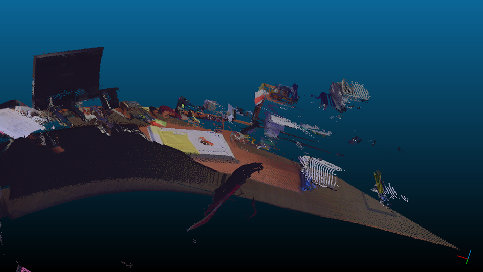
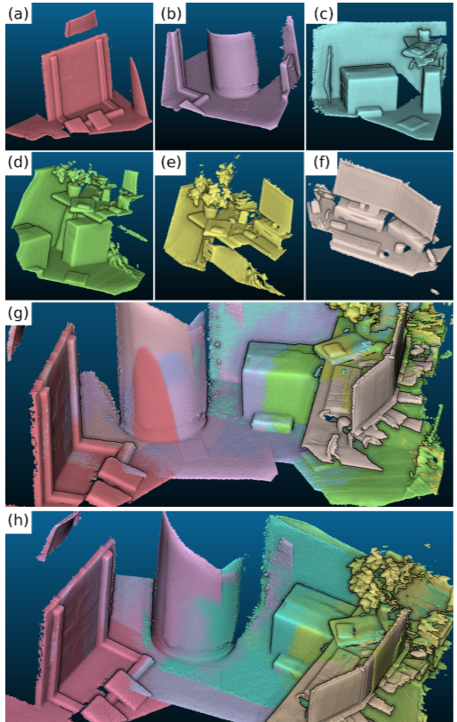
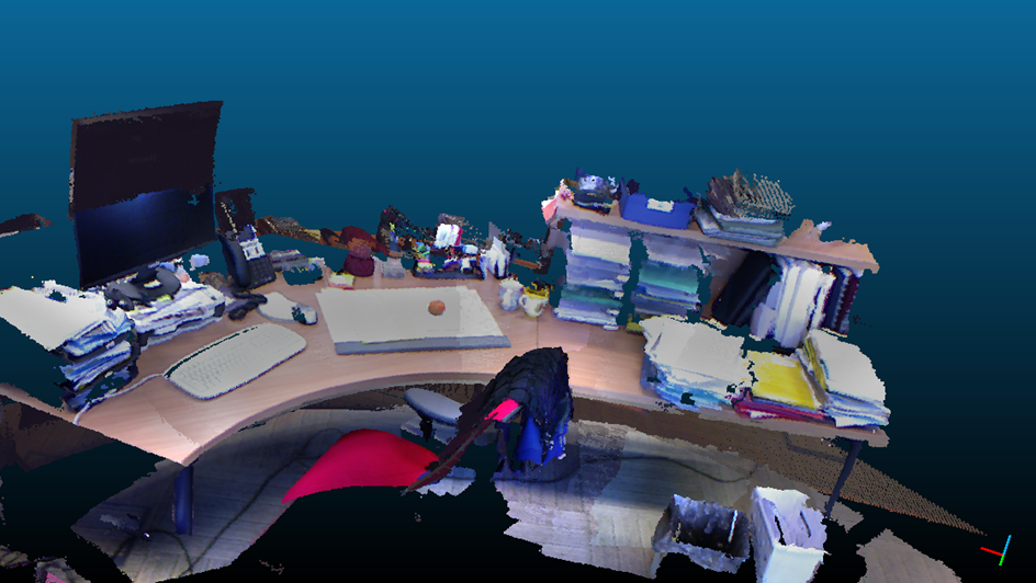
LiDAR scan of an indoor scene: accurate global structure, but sparse with many holes from occlusions.

RGB-D sensor frames: very dense and colorful local reconstructions, limited to about 4.5 m range.

Property	LiDAR	Kinect
Accuracy	High (mm-level)	Low–Medium
Density	Low (sparse)	High (dense)
Scale	Global	Local
Holes	Many (occlusions)	Few (within range)
Color	Limited	Full RGB
Cost	Expensive	Inexpensive

Result of fusing LiDAR and Kinect data: holes in the LiDAR scan are filled with dense Kinect geometry.

4. Three-Stage Multi-Modal Fusion Pipeline

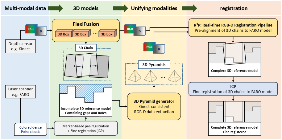
Fusing LiDAR and Kinect data follows three sequential stages:

Stage	Goal	Key Technique
Stage 1	Unify data format representation	3D pyramid decomposition + raycasting
Stage 2	Unify coordinate space	SIFT feature matching, transformation chain
Stage 3	Fuse into unified 3D model	TSDF integration or point cloud merge

5. Stage 1: Unifying Data Format

Goal

Bring both LiDAR and Kinect data to a unified format — preferably RGB-D — so that 2D image-based matching can be applied. Full 3D formats (point cloud, voxel grid) are computationally expensive for matching.

3D Pyramid Decomposition

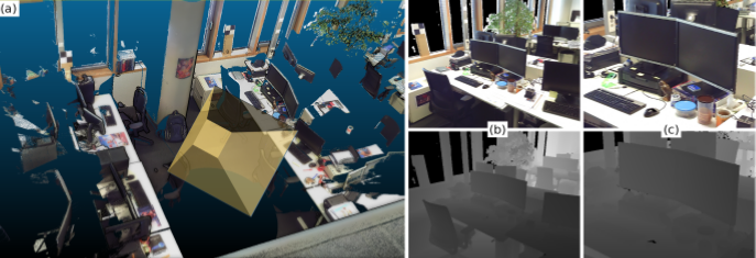
This is the key technique for converting a LiDAR point cloud into a set of virtual RGB-D frames:

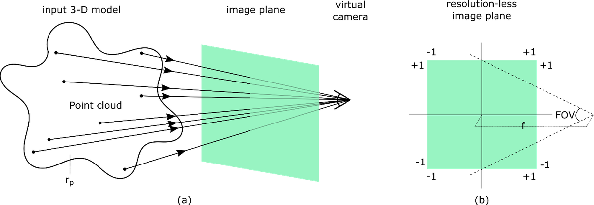
Decompose the point cloud into 3D pyramids — frustum-shaped volumes representing virtual camera viewpoints. Each pyramid's shape is designed to match the Kinect's intrinsic parameters (FOV, focal length, aspect ratio).
Generate synthetic RGB-D images via raycasting — a virtual camera is placed at the pyramid apex. Rays cast through an image plane into the point cloud produce a synthetic depth image and synthetic RGB image per pyramid.
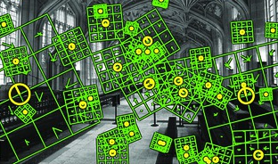
Compute SIFT features on each synthetic RGB image for later matching against real Kinect frames.

3D pyramid decomposition: frustum-shaped virtual camera viewpoints placed over the LiDAR point cloud. Each pyramid generates a virtual RGB-D view.

Raycasting geometry: rays cast from the input point cloud through a normalized image plane $[-1, +1]$ to a virtual camera, generating synthetic depth and RGB images.

SIFT keypoints detected on a synthetic RGB image generated from the LiDAR point cloud, ready for matching against Kinect frames.

Why convert LiDAR to RGB-D format?

By converting LiDAR data to synthetic RGB-D views that use the same camera model as the Kinect, we can use standard 2D feature matching (SIFT) to establish correspondences. This is computationally far cheaper than direct 3D point cloud registration.

6. Stage 2: Unifying the Coordinate Space

Master Coordinate System

The LiDAR coordinate system is adopted as the master coordinate system. All virtual pyramids were defined on the LiDAR point cloud, so their poses in the LiDAR frame are already known.

Registration via SIFT Feature Matching

For each real Kinect RGB-D frame:

Compute SIFT features on the Kinect's RGB image.
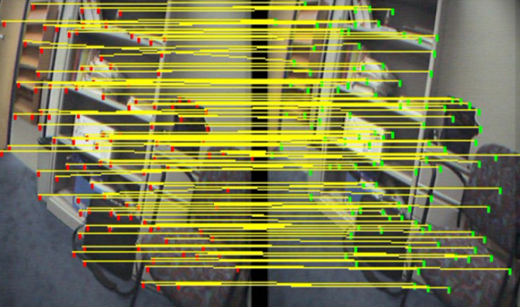
For each pyramid's synthetic image, find SIFT feature correspondences with the Kinect image (ratio test + RANSAC).
If correspondences are found below an error threshold, compute the transformation matrix $[R | \mathbf{t}]$ from Kinect frame to pyramid coordinate system.
Since the pyramid's pose in the master system is known, compute the Kinect frame's pose in the master system.

SIFT matching between Kinect and pyramid views

SIFT feature correspondences between a real Kinect RGB image and a synthetic pyramid image. Colored lines connect matched keypoints.

Transformation Chain

$$T_{\text{Kinect} \to \text{master}} = T_{\text{pyramid} \to \text{master}} \cdot T_{\text{Kinect} \to \text{pyramid}}$$ The first term is known (pyramid defined on LiDAR cloud); the second is computed from SIFT correspondences.

7. Stage 3: Fusing into a Unified 3D Model

Option A: TSDF Volume Fusion

Project both RGB-D pyramids (from LiDAR raycasting) and Kinect samples (from their known master poses) onto a global TSDF voxel grid. The TSDF update rule naturally fuses both data sources via weighted averaging:

TSDF Update Rule

$$\text{TSDF}_{\text{new}}(\mathbf{x}) = \frac{\text{TSDF}_{\text{old}}(\mathbf{x}) \cdot w_{\text{old}}(\mathbf{x}) + d_{\text{meas}} \cdot w_{\text{new}}}{w_{\text{old}}(\mathbf{x}) + w_{\text{new}}}$$ Positive TSDF: free space in front of surface. Negative: inside object. Zero crossing: the surface.

Option B: Point Cloud Fusion

Extract a point cloud from each Kinect RGB-D frame using the back-projection formula:

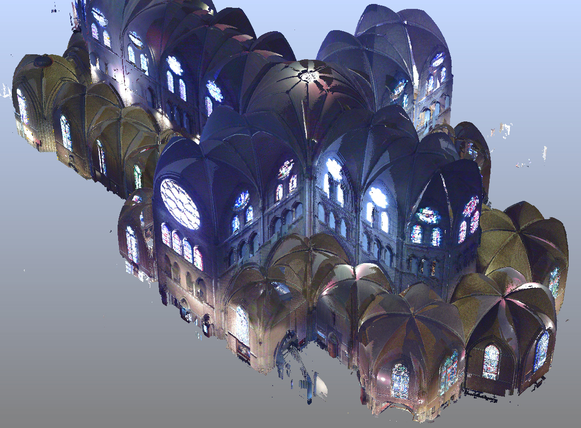
\mathbf{P}_{3D} = \begin{bmatrix} (u - c_x) \cdot d / f_x \\ (v - c_y) \cdot d / f_y \\ d \end{bmatrix}

Transform into the master coordinate system, merge with the LiDAR point cloud, then filter for outliers and duplicates using octree-based deduplication.

Criterion	TSDF Fusion	Point Cloud Fusion
Noise handling	Natural averaging	Requires post-processing
Memory	Fixed $O(N^3)$ grid	Scales with point count
Lossy/Lossless	Lossy	Lossless
Error recovery	Difficult (baked in)	Easier (remove bad sets)
Best for	Dense room-scale reconstruction	Large-scale sparse environments

Result of multi-modal fusion: a cathedral interior reconstruction combining LiDAR global accuracy with dense Kinect geometry.

8. KinectFusion Limitations

KinectFusion is a real-time 3D reconstruction system using ICP-based pose tracking integrated into a TSDF voxel grid. It has three major practical limitations:

Limitation	Root Cause	Consequence
Limited TSDF volume size	GPU memory constraints	Cannot reconstruct environments larger than ~3×3×3 m
ICP requires slow motion	Point correspondences fail on large displacements	Camera must move slowly and smoothly
Drift causes geometry melting	No loop closure; ICP error accumulates	Surfaces blur and distort permanently

Key insight — TSDF is lossy

Once depth data is integrated at a wrong position due to drift, the error is permanent. The weighted average bakes the error into the voxel values and individual frames cannot be recovered from the volume.

9. Limitation 1: TSDF Volume Size — Rolling Buffer

The Problem

A $512^3$ TSDF grid covers only ~3×3×3 meters and requires ~2 GB GPU memory. A $1024^3$ grid requires ~8.6 GB — often too large for real-time processing:

\text{Memory} = N^3 \times B \text{ bytes}

where $N$ is the grid resolution per dimension and $B$ is bytes per voxel (typically 8–16 bytes).

A TSDF volume is a fixed-size 3D cube (e.g., 512×512×512 voxels covering 3×3×3 m). GPU memory limits the cube size.

Rolling Buffer (Kintinuous)

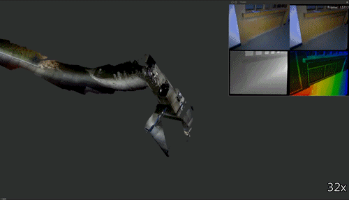
Kintinuous introduces a rolling buffer to allow unbounded spatial extent while keeping GPU memory constant:

Maintain the TSDF volume at its original GPU size (e.g., $512^3$).
As the camera moves forward, offload the spatial region the camera has already passed (~30 cm offset) to CPU/system memory.
Clear those voxels in the GPU volume.
Create new empty TSDF space (~30 cm) in the camera's direction of movement.

Kintinuous: real-time 3D reconstruction using a rolling buffer. GPU memory stays constant while the accumulated model can grow unboundedly.

10. Limitation 2: Drift and Geometry Melting

What is Drift?

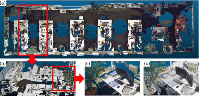
Drift = accumulated erroneous pose estimation over time. In KinectFusion, each ICP iteration introduces a small pose error $\epsilon_i$. These accumulate:

\text{Total drift after } N \text{ frames} \approx \sum_{i=1}^{N} \epsilon_i

Why Drift Causes Melting

When the camera pose estimate is wrong:

The new depth image is projected onto the TSDF volume at a slightly incorrect position.
The TSDF integration averages the new (misaligned) measurements with existing (correct) ones.
The signed distance field contains contradictory measurements at the zero-crossing.
The surface becomes blurred, doubled, or distorted — this is called "melting."

Recovery is nearly impossible: TSDF is lossy — the weighted average permanently corrupts voxel values. As more frames are integrated with accumulating drift, the corrupted model also degrades future ICP tracking — a vicious cycle.

Drift in KinectFusion: reconstruction becomes distorted as ICP pose errors accumulate. Visible doubling and blurring of surfaces ("melting") appear after short camera movements.

11. Solution A: Chained TSDF Boxes

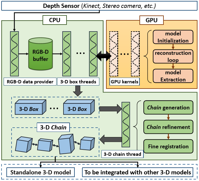
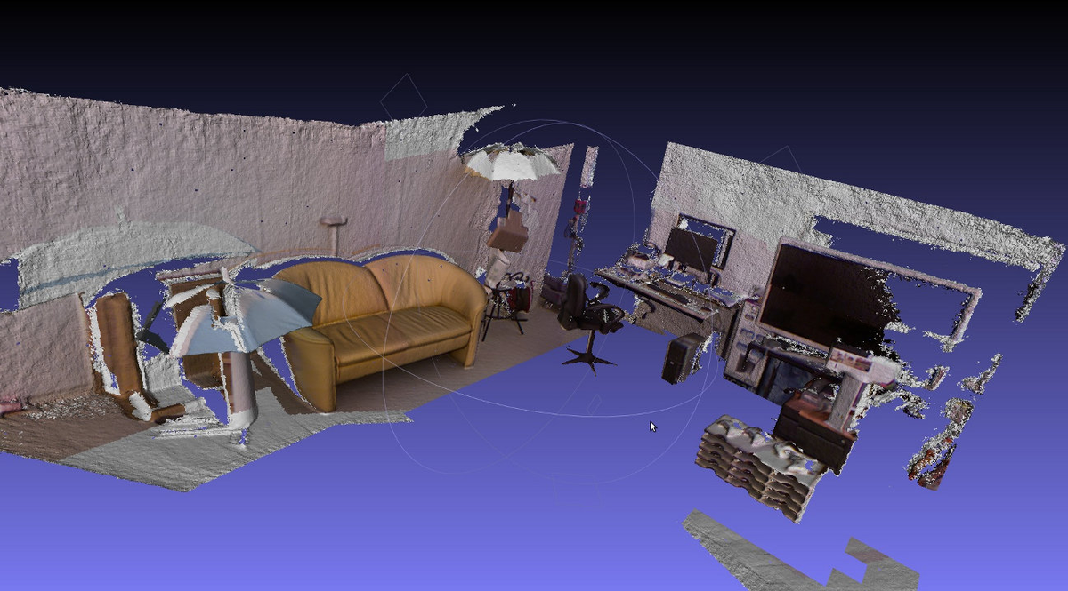
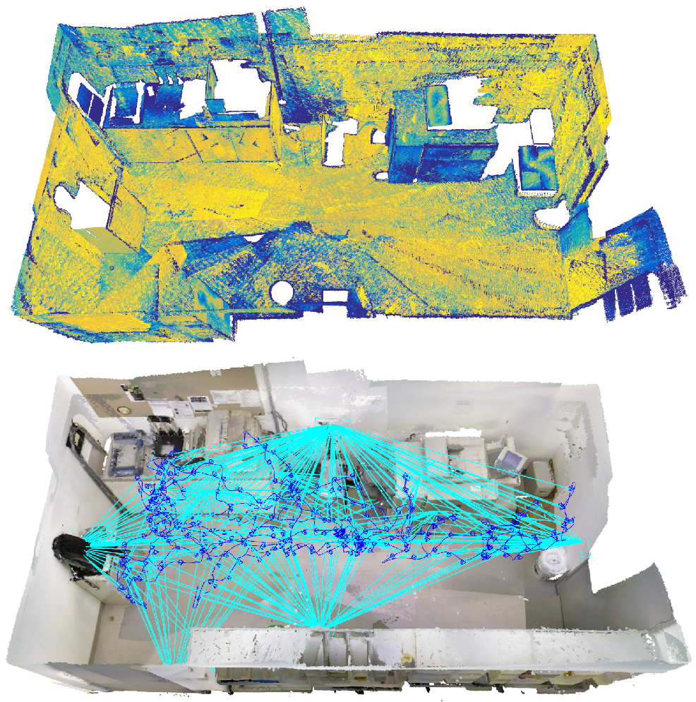
Instead of one continuous TSDF volume for the entire session, create a chain of separate TSDF boxes, each covering a short time window (~10 seconds). Within each box, drift is minimal. After capture, all boxes are combined into one global model.

Aspect	Detail
Local drift	Minimal — each box has short accumulation time
Global drift	Not corrected — boxes themselves may be misaligned
Loop closure	Not possible — boxes are independent during capture

Chained TSDF pipeline: CPU manages RGB-D data provider and box threads; GPU handles bilateral filtering, vertex/normal computation, ICP, TSDF generation, raycasting, and free registration between boxes.

Chained TSDF boxes merged into a global model: each box is a clean local reconstruction combined into a room-scale result.

12. Solution B: Plane-Based Drift Correction

Method

From every depth keyframe (~every 30 frames), detect large planar surfaces: walls, floor, ceiling, large furniture.
Match these planes keyframe-to-keyframe using plane parameters (normal direction $\mathbf{n}$, distance $d$).
With 3 matched non-parallel plane pairs, correct all 6 DoF of pose error: translation $(T_x, T_y, T_z)$ and rotation $(R_x, R_y, R_z)$.

Plane Equation

$$\mathbf{n} \cdot \mathbf{p} + d = 0, \qquad \mathbf{n} = (n_x, n_y, n_z), \quad \|\mathbf{n}\| = 1$$

Why It Resembles Loop Closure — but Better

Loop closure requires the camera to physically revisit a location. Plane-based correction uses persistent structural features (walls, floors) visible from many viewpoints — drift can be corrected at every keyframe, far more frequently than loop closure opportunities arise.

Plane-based drift correction: reconstructed apartment colored by surface orientation (yellow = horizontal, blue = vertical). Camera trajectory overlaid in cyan.

Complete 3D sensing and reconstruction pipeline: multi-modal data flows from raw sensor capture through format unification, coordinate alignment, and into a final fused 3D model.

13. SVD-Based Pose Estimation

Given $N$ pairs of corresponding 3D points $\{(\mathbf{p}_i, \mathbf{q}_i)\}$, find the rigid transformation (rotation $R$ and translation $\mathbf{t}$) that aligns source points to target points:

E(R, \mathbf{t}) = \sum_{i=1}^{N} \| \mathbf{q}_i - (R \cdot \mathbf{p}_i + \mathbf{t}) \|^2

SVD Registration Summary

Centroids: $\bar{\mathbf{p}} = \frac{1}{N}\sum \mathbf{p}_i$, $\quad \bar{\mathbf{q}} = \frac{1}{N}\sum \mathbf{q}_i$

Cross-covariance: $H = \sum_{i=1}^{N} (\mathbf{p}_i - \bar{\mathbf{p}})(\mathbf{q}_i - \bar{\mathbf{q}})^T$

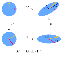
SVD: $H = U \Sigma V^T$

Optimal rotation: $R = V U^T$ (if $\det(VU^T) = -1$, negate the column of $V$ for smallest singular value)

Translation: $\mathbf{t} = \bar{\mathbf{q}} - R \bar{\mathbf{p}}$

Geometric interpretation of SVD: matrix $M$ decomposed into rotation $V^*$ (aligns data to principal axes), scaling $\Sigma$, and rotation $U$ (maps to target space). $M = U \Sigma V^*$.

Property	Detail
Optimal	Minimizes sum of squared distances (least-squares optimal)
Closed-form	No iterative optimization needed
Requires	Known point correspondences; minimum 3 non-collinear pairs
Use in ICP	ICP iterates: find correspondences → compute SVD → apply transform → repeat

Flashcards

← 10. Autoencoders 12. Data Analysis →