10. Autoencoders

Encoder-decoder architecture, bottleneck, denoising AE, convolutional AE, anomaly detection

Contents

1. Anomaly Detection in Computer Vision 2. Anomaly Detection as Outlier Detection 3. Autoencoders: Core Concept 4. Architecture: Encoder, Bottleneck, Decoder 5. Anomaly Detection with Autoencoders 6. Denoising Autoencoders 7. Convolutional Autoencoders (CAE) 8. Pooling, Unpooling, and Deconvolution 9. Autoencoder Hyperparameters 10. Loss Functions 11. Variational Autoencoders (VAE) Interactive: Autoencoder Architecture Flashcards

1. Anomaly Detection in Computer Vision

Anomaly detection is the task of identifying events, observations, or data points that deviate significantly from expected "normal" behavior. In computer vision, this applies to detecting unusual events in images or video streams.

Well-Defined Anomalous Events

Some anomalies are specific and definable:

Violence detection — identifying physical altercations in surveillance footage.
Loitering — detecting people who remain in an area for an unusually long time.
Traffic rule violations — cars running red lights, wrong-way driving, etc.

The Fundamental Challenge

Real-world anomalies are far more complicated. The core problem: it is not easy (or even possible) to list all possible anomalous behaviors. You cannot train a simple classifier because anomalies are, by definition, rare and unpredictable. A new type of anomaly may appear that was never seen in training data.

The solution: model normality

Instead of enumerating all anomalies, learn what "normal" looks like from normal-only training data. At test time, check how well new data matches the model of normality. Significant mismatch = anomaly. This is one-class learning or novelty detection.

2. Anomaly Detection as Outlier Detection

The implementation follows these steps:

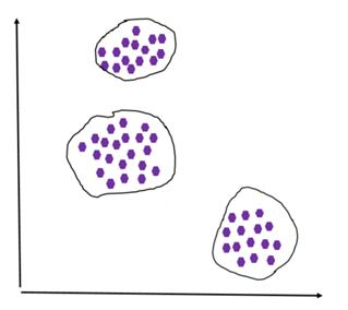
Represent events as points in a high-dimensional feature space. Both normal and anomalous events are transformed into feature vectors $\mathbf{f} = [x_1, x_2, \ldots]$ by a feature extraction model.
Model the "normal" using training data. Only normal examples are used during training. These form clusters in feature space.
Declare statistically unlikely points as anomalies. At test time, new points that fall far from the learned clusters are anomalies.

Anomaly detection as outlier detection in feature space

Normal data (purple dots) forms tight clusters in feature space. Normal test samples (green) fall within clusters; anomalies (red) appear as outliers far from any cluster.

Key principle

The model never sees anomalies during training. It only learns what "normal" looks like. Anything that does not fit is flagged as an anomaly.

3. Autoencoders: Core Concept

Definition — Autoencoder

An autoencoder is a neural network trained to reconstruct its own input. The input and output are desired to be the same; the network minimizes the difference between them.

The Bottleneck Constraint

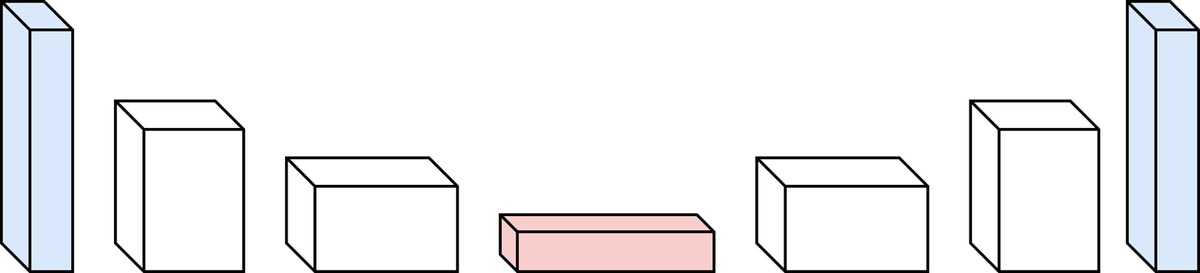
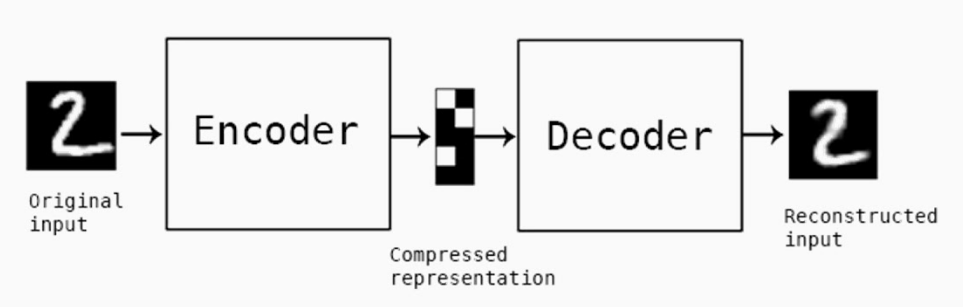
An autoencoder is forced to pass all information through a compressed representation — called the bottleneck, code, or latent space — that has far fewer dimensions than the input. This prevents a trivial identity-function solution and forces the network to:

Compress the input into its most essential features (encoding).
Reconstruct the input from only those essential features (decoding).

Types of Autoencoders

Type	Description
Vanilla	Fully-connected (dense) layers only
Stacked	Multiple layers in both encoder and decoder
Convolutional (CAE)	Convolutional and deconvolutional layers; good for images/video
Denoising	Trained to reconstruct clean inputs from noisy versions
Variational (VAE)	Encoder outputs a distribution; enables generation

Applications

Anomaly detection (primary focus of this module)
Image reconstruction and denoising
Dimensionality reduction (nonlinear alternative to PCA)
Feature learning (bottleneck representations as features)
Recommendation systems

4. Architecture: Encoder, Bottleneck, Decoder

The Encoder

The encoder takes the high-dimensional input and progressively reduces its dimensionality through successive layers (each with fewer nodes than the previous). It produces the compressed latent representation at the bottleneck, finding the fundamental information in the input and stripping away noise.

z = f_{\text{encoder}}(x)

The Bottleneck

The narrowest layer — with the fewest nodes. It holds the most compressed version of the input that the network has learned. The bottleneck dimension is a critical hyperparameter:

Smaller: more compression, more information loss, but forces the network to learn only the most essential features.
Larger: less compression, better reconstruction, but the network may learn a near-identity mapping without meaningful features.

The Decoder

The decoder takes the bottleneck representation and progressively increases dimensionality through layers with increasing numbers of nodes, producing the reconstructed input.

\hat{x} = f_{\text{decoder}}(z)

Complete Autoencoder

$$\hat{x} = f_{\text{decoder}}(f_{\text{encoder}}(x))$$
Training objective: minimize the difference between $x$ and $\hat{x}$ via backpropagation.

Stacked autoencoder architecture with bottleneck and MSE loss

Stacked autoencoder: encoder blocks get progressively smaller, the bottleneck (pink) is the narrowest, decoder blocks expand symmetrically. MSE loss is computed between input and output.

Encoder-decoder block diagram with MNIST digits

A clean MNIST digit passes through the Encoder to a compressed representation, then the Decoder reconstructs it. The autoencoder is trained to make the output match the input.

5. Anomaly Detection with Autoencoders

The Core Idea

Train the autoencoder on only normal data. The encoder learns to compress normal patterns; the decoder learns to reconstruct them.
At test time, feed new data through the autoencoder.
- Normal input: reconstructed well, low reconstruction error.
- Anomalous input: reconstructed poorly, high reconstruction error — the model has never learned patterns of anomalies.
Threshold the reconstruction error to classify as normal or anomalous.

Anomaly Score and Decision Rule

$$\text{score}(x) = \| x - \hat{x} \|^2 = \| x - f_{\text{decoder}}(f_{\text{encoder}}(x)) \|^2$$ $$\text{decision}(x) = \begin{cases} \text{anomaly} & \text{if } \text{score}(x) > \tau \\ \text{normal} & \text{otherwise} \end{cases}$$

Why this works

The bottleneck forces the autoencoder to learn a compact representation of what "normal" looks like. When an anomaly arrives, the learned representation does not capture its unusual features. The decoder reconstructs something "normal" instead, and the mismatch with the actual anomalous input produces a high reconstruction error.

6. Denoising Autoencoders

Definition — Denoising Autoencoder

A denoising autoencoder is trained to predict the original clean input from a corrupted (noisy) version of that input.

Training Procedure

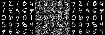
Start with clean training data $x$.
Add noise: $\tilde{x} = x + \text{noise}$ (typically white/Gaussian noise).
Feed the noisy input $\tilde{x}$ through the autoencoder to produce reconstruction $\hat{x}$.
Compute loss between the reconstruction $\hat{x}$ and the original clean input $x$ (not the noisy input!).

Denoising Autoencoder Loss

$$\mathcal{L} = \| x - f_{\text{decoder}}(f_{\text{encoder}}(\tilde{x})) \|^2$$
Target is the clean original $x$, not the noisy input $\tilde{x}$.

Denoising autoencoder MNIST example: original, noisy, and reconstructed digits

Denoising autoencoder applied to MNIST: clean original digits (left), noisy corrupted versions (center), clean reconstructed outputs (right).

Aspect	Standard Autoencoder	Denoising Autoencoder
Input to encoder	Clean $x$	Noisy $\tilde{x}$
Loss target	Clean $x$	Clean $x$ (same)
Training signal	Reconstruct input	Reconstruct clean from noisy

Key insight for anomaly detection

The denoising autoencoder learns to reconstruct normal, clean patterns even from corrupted inputs. When it encounters an anomaly, the reconstruction loss is significantly higher than for normal examples — because the model has only learned to reconstruct normal patterns. This elevated loss serves as the anomaly signal.

7. Convolutional Autoencoders (CAE)

Most state-of-the-art anomaly detection methods in video use Convolutional Autoencoders (CAEs), which replace fully-connected layers with convolutional and deconvolutional layers.

Why CAEs?

Spatial structure exploitation: Convolutions preserve and exploit 2D spatial relationships, unlike vanilla AEs that treat each pixel independently.
Weight sharing: Convolutional kernels are applied everywhere — far fewer parameters than fully-connected layers.
Translation invariance: Built into the convolutional operation.
Scalability: Scales well to large images/video.
Reconstruction quality: CAEs are notably good at reconstructing images from lower-dimensional latent features.

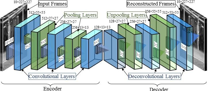
CAE architecture: convolutional/pooling layers in the encoder (left) progressively reduce spatial dimensions. Corresponding unpooling/deconvolutional layers in the decoder (right) restore them. MSE loss is computed between input and output frames.

CAE Architecture Example

Side	Operations	Dimensions (example)
Encoder	Input frames	$10 \times 227 \times 227$
Encoder	Conv + Pool (repeated)	$512 \times 55 \times 55 \to 256 \times 13 \times 13$
Latent features (bottleneck)		Compressed representation
Decoder	Unpool + Deconv (repeated)	$128 \times 13 \times 13 \to 256 \times 55 \times 55$
Decoder	Output frames	$10 \times 227 \times 227$

Key design principle

The dimensionality of the input and output must be the same. Everything in between (the bottleneck and the depth/width of encoder/decoder) can be adjusted as a hyperparameter.

Aspect	Vanilla Autoencoder	Convolutional Autoencoder
Layer type	Fully-connected (dense)	Conv + Pooling / Deconv + Unpooling
Spatial structure	Ignored; input flattened	Preserved via convolutions
Parameter count	Very large (all pixels connected)	Small (weight sharing via kernels)
Translation invariance	Not inherent	Built-in
Best for	Small, non-spatial data	Images, video, spatial data

8. Pooling, Unpooling, and Deconvolution

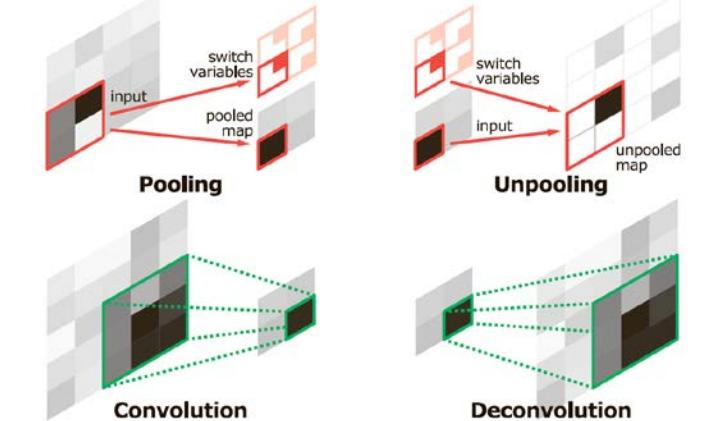
For each convolutional layer in the encoder there is a corresponding deconvolutional layer in the decoder. For each pooling layer there is a corresponding unpooling layer.

Max-Pooling (Encoder Side)

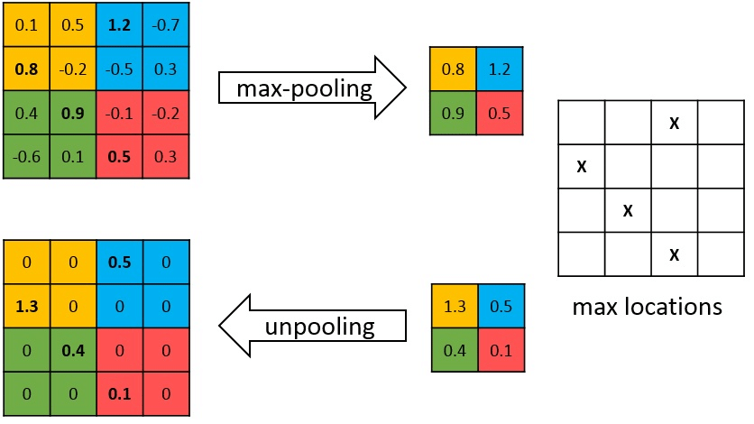
Downsamples by selecting the maximum value from each local region. A $2 \times 2$ max-pool with stride 2 reduces a $4 \times 4$ map to $2 \times 2$.

Max-pooling reduces a 4x4 input to 2x2 by taking the maximum of each 2x2 block. The locations of the maxima are stored as switch variables for later unpooling.

Switch Variables (Stored Max Locations)

During max-pooling, the locations (indices) of the maximum values are stored. These are called switch variables. Without these stored locations, the decoder would not know where to place values during upsampling.

Unpooling (Decoder Side)

Reverses max-pooling by placing values back at their original max locations (from the stored switch variables) and filling all other positions with zeros.

Numerical example: max-pooling and unpooling

Input (4×4):

0.1	0.5	1.2	-0.7
0.8	-0.2	-0.5	0.3
0.4	0.9	-0.1	-0.2
-0.6	0.1	0.5	0.3

After 2×2 max-pool (stride 2): output (2×2)

0.8 (row 1, col 0)	1.2 (row 0, col 2)
0.9 (row 2, col 1)	0.5 (row 3, col 2)

Unpooling with values [1.3, 0.5; 0.4, 0.1] placed at stored max locations:

0	0	0.5
1.3	0	0
0	0.4	0
0	0	0.1

Values are placed at the stored max locations; all other positions are zero.

Deconvolution (Transposed Convolution)

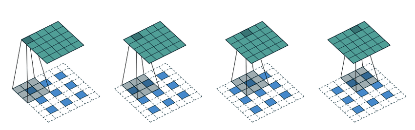
A transposed convolution (deconvolution) recovers spatial resolution from compressed features. Where a regular convolution maps many input elements to one output element (many-to-one), a transposed convolution maps each input element to multiple output elements (one-to-many), effectively spreading information to a larger spatial map.

Transposed convolution (deconvolution) upsampling: a smaller feature map is expanded to a larger spatial resolution by spreading each input element to multiple output elements.

Comparison of pooling/unpooling and convolution/deconvolution

Comparison: (top) pooling with switch variables and unpooling; (bottom) convolution (many-to-one) vs. deconvolution (one-to-many).

9. Autoencoder Hyperparameters

There are 4 key hyperparameters that must be set before training an autoencoder:

Hyperparameter	Description	Effect of extremes
Code size (bottleneck dimension)	Number of nodes in the middle layer	Too small: excessive compression, poor reconstruction even for normal data. Too large: near-identity mapping, no meaningful features learned.
Number of layers (depth)	How many layers in encoder and decoder (not counting input/output)	Too shallow: cannot learn complex hierarchical features. Too deep: vanishing gradients, overfitting, training difficulty.
Nodes per layer (width)	Neurons per layer; decreases in encoder, increases in decoder (symmetric)	Too few: information bottleneck at multiple points. Too many: excessive parameters, overfitting.
Loss function	Typically MSE; measures reconstruction quality	Wrong choice (e.g., MSE for binary data instead of binary cross-entropy): suboptimal training and poor reconstruction quality.

Symmetry principle

The decoder is symmetric to the encoder: if the encoder has layers with 256, 128, 64 nodes, the decoder has layers with 64, 128, 256 nodes. This symmetry is a standard design choice, not a strict mathematical requirement.

10. Loss Functions

Mean Squared Error (MSE)

MSE Loss

$$\mathcal{L}_{\text{MSE}} = \frac{1}{N} \sum_{i=1}^{N} (x_i - \hat{x}_i)^2$$

Mean Absolute Error (MAE / L1)

\mathcal{L}_{\text{MAE}} = \frac{1}{N} \sum_{i=1}^{N} |x_i - \hat{x}_i|

Loss for Denoising Autoencoders

The loss is computed between the reconstruction and the clean original, not the noisy input that was fed to the encoder:

\mathcal{L} = \| x - f_{\text{decoder}}(f_{\text{encoder}}(\tilde{x})) \|^2

MSE vs. MAE for anomaly detection

MSE penalizes large errors more heavily (quadratic), making it more sensitive to strongly anomalous pixels. This can be beneficial for anomaly detection — large deviations get disproportionately large scores.

MAE treats all errors equally (linear), making it more robust to a few large outliers but potentially less sensitive to localized anomalies. The CAE formula shown in the lecture, $l(x,y) = \frac{1}{N}\sum\sqrt{(x_n - y_n)^2}$, is equivalent to MAE.

11. Variational Autoencoders (VAE)

Standard autoencoders learn a deterministic mapping to a potentially discontinuous, unstructured latent space. A Variational Autoencoder (VAE) addresses this by making the encoder produce a probability distribution over latent space rather than a single point.

VAE Encoder

Instead of mapping input $x$ to a single latent vector $z$, the encoder maps $x$ to the parameters of a Gaussian distribution:

\mu = f_\mu(x), \quad \log \sigma^2 = f_{\sigma}(x)

The latent vector is then sampled: $z \sim \mathcal{N}(\mu, \sigma^2)$.

The Reparameterization Trick

Sampling from $\mathcal{N}(\mu, \sigma^2)$ is a stochastic operation that breaks the backpropagation chain. The reparameterization trick rewrites sampling as:

Reparameterization Trick

$$z = \mu + \sigma \odot \epsilon, \quad \epsilon \sim \mathcal{N}(0, I)$$
The randomness is externalized to $\epsilon$ (which has no network parameters). Gradients can flow through the deterministic $\mu$ and $\sigma$ back to the encoder weights, enabling end-to-end backpropagation.

VAE Loss Function

VAE Loss

$$\mathcal{L}_{\text{VAE}} = \mathcal{L}_{\text{reconstruction}} + \mathcal{L}_{\text{KL}}$$ $$\mathcal{L}_{\text{KL}} = D_{\text{KL}}(q(z|x) \| p(z)) = -\frac{1}{2} \sum_{j=1}^{J} \left(1 + \log(\sigma_j^2) - \mu_j^2 - \sigma_j^2 \right)$$

Role of the KL Divergence Term

The KL divergence regularizes the latent space by forcing the learned distribution $q(z|x) = \mathcal{N}(\mu, \sigma^2)$ toward the standard normal prior $p(z) = \mathcal{N}(0, I)$:

Regularization: Prevents the encoder from mapping each input to a completely different, disconnected region.
Continuity: Similar inputs map to nearby points in latent space.
Completeness: Every point in latent space, when decoded, produces a meaningful output.
Generation: You can sample $\epsilon \sim \mathcal{N}(0, I)$ and decode to generate new data.

What happens without the KL term?

Without the KL divergence term, the VAE degenerates into a standard autoencoder. The encoder learns to map each input to very small-variance point estimates in disconnected regions of latent space. This leads to a discontinuous latent space with gaps, no ability to generate meaningful new data by sampling, and no regularization (the model may overfit to training data).

VAE vs. standard AE for anomaly detection

VAEs can be used for anomaly detection similarly to standard autoencoders, but with an additional signal: both the reconstruction error and the KL divergence can indicate anomalies. Anomalous inputs may have both high reconstruction error and unusual latent distributions (high KL divergence).

Flashcards

← 10. SLAM 11. Data Fusion →