13. Behaviour Analysis

Action recognition, optical flow, I3D, SlowFast, anomaly detection, autoencoders

Contents

1. Problem Definition and Applications 2. Action Recognition 3. Two-Stream Architecture 4. 2D vs. 3D Convolutions 5. CNN + LSTM for Video 6. Outlier-Based Anomaly Detection 7. Autoencoders for Anomaly Detection 8. Convolutional Autoencoders (CAEs) 9. I3D Architecture 10. Multiple Instance Learning 11. SlowFast Architecture 12. Crowd Behaviour Analysis Interactive: I3D Walkthrough Flashcards

1. Problem Definition and Applications

Behaviour analysis in computer vision aims to extract high-level semantic behavior information from a scene, typically from video. It goes beyond detecting what objects are present to understanding what those objects are doing.

Why It Is Needed

Increased video data availability: Surveillance cameras, dashcams, and smartphones generate far more video than humans can analyze. The volume is growing faster than the workforce that can monitor it.
Automation requirement: Security monitoring, traffic management, and sports analytics all require automatic behavior interpretation.
Context-dependence: The same motion can mean different things depending on scene context (running at a track vs. running from a crime scene).

Application	Description
Surveillance	Monitoring public or private spaces for security threats
Anomaly detection	Identifying unusual or suspicious events (abandoned bags, erratic behavior)
Violence detection	Detecting fighting, assault, or violent actions automatically
Traffic monitoring	Analyzing vehicle and pedestrian flow, detecting violations
Video content analysis	Scanning uploaded videos for illegal content (used by video platforms and law enforcement)
Sports event detection	Automatically detecting goals, fouls, and other events
Crowd analysis	Panic detection, crowd counting, anomalous flow detection

2. Action Recognition

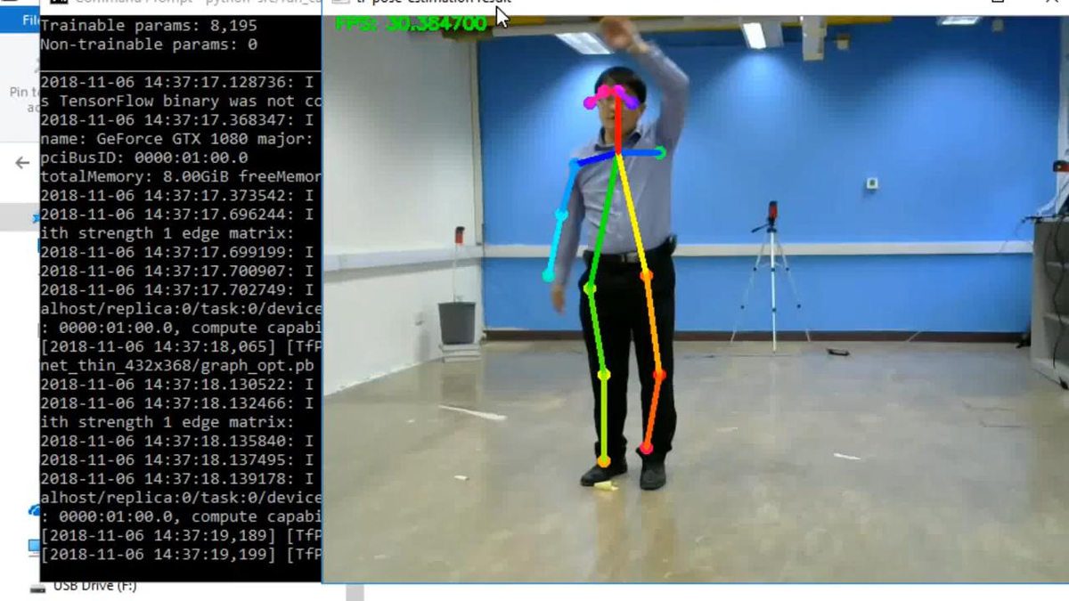
Action/activity recognition determines the activity a person is doing. In the supervised variant this is a classification problem where the set of possible actions is pre-defined (e.g., walking, running, jumping).

Pose estimation skeleton overlay used for action recognition: colored skeleton drawn on the body to classify the activity.

Still Images vs. Video

Input	Difficulty	Approach
Still images	Relatively simple classification problem	Standard CNNs; single-frame appearance features
Video	Added temporal dimension makes problem harder	3D CNNs, RNN/LSTM, two-stream architectures

Key insight

Feature extraction is the most important part of action recognition, especially for videos. Temporal information — how the scene changes over time — carries crucial information that single-frame analysis cannot capture.

3. Two-Stream Architecture

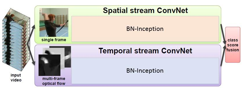
The two-stream architecture handles video by splitting spatial and temporal processing into two parallel CNN pathways:

Two-stream ConvNet: spatial stream (single RGB frame) and temporal stream (multi-frame optical flow) processed in parallel, scores fused for final prediction.

Stream	Input	Captures
Spatial stream	Single RGB frame	Appearance: what objects look like, scene context, body pose
Temporal stream	Multi-frame optical flow	Motion: how objects are moving

Optical flow (a simplified approach to handling the temporal dimension) transforms the 3D video into 2D motion history by collapsing the temporal dimension into flow fields. The spatial and temporal class scores are then fused (e.g., by averaging or learned weighting) to produce the final action prediction.

4. 2D vs. 3D Convolutions

Comparison of 2D convolution (on image and multiple channels) vs. 3D convolution (on volume and multiple channels).

Property	2D Convolution on video	3D Convolution on video
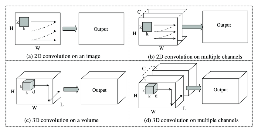
Kernel shape	$k \times k$ (spatial only)	$k \times k \times d$ (spatial + temporal)
Sliding dimensions	Height, width only	Height, width, AND time
Output	2D feature map per frame	3D feature volume
Temporal modeling	Treats frames independently	Learns spatiotemporal features jointly

3D Convolution on Video

$$\text{Output}(i,j,t) = \sum_{m}\sum_{n}\sum_{\tau} \text{Input}(i+m, j+n, t+\tau) \cdot \text{Kernel}(m,n,\tau)$$ The temporal extent $d$ of the 3D kernel determines how many consecutive frames are jointly processed. 3D CNNs learn spatiotemporal features that 2D CNNs applied frame-by-frame cannot capture.

5. CNN + LSTM for Long-Term Temporal Dependencies

3D CNNs have trouble with long-term temporal dependencies (e.g., understanding that a high jump involves a run-up, jump, and landing spread over many seconds). The CNN + LSTM pipeline addresses this:

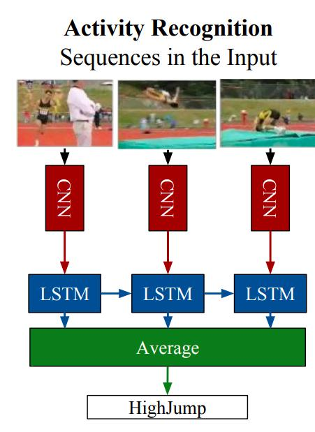
CNN + LSTM pipeline: per-frame CNN features fed sequentially into an LSTM, averaged for final classification.

CNN: Extracts a feature vector from each individual frame.
LSTM: Processes the sequence of per-frame feature vectors, maintaining a hidden state that accumulates temporal information.
Average: LSTM outputs are averaged to produce a single clip-level feature vector.
Classification: The clip-level feature is classified into an action category.

Sequence Model	Key Property
RNN	Basic recurrent model; suffers from vanishing/exploding gradients for long sequences
GRU	Uses update and reset gates; simpler than LSTM; good for moderate-length sequences
LSTM	Input, output, and forget gates; excels at long-term dependencies

6. Outlier-Based Anomaly Detection

Detecting specific anomalies with supervised classifiers is possible but requires enumerating all possible anomalies. Real-world anomalies are too diverse for this. The better approach: model the normal and detect deviations.

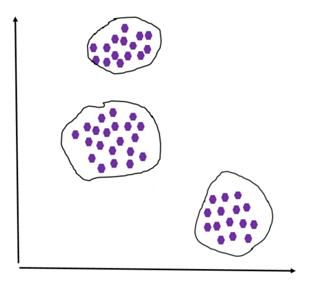
Outlier detection: normal training data (purple) forms clusters in feature space. New test points near clusters are normal (green); points far from clusters are anomalies (red).

Training: Represent events as points in high-dimensional feature space. Model what "normal" looks like using only normal training data.
Testing: Evaluate model mismatch — events far from the learned normal distribution are declared anomalies.

Key insight

It is impossible to enumerate all possible anomalies, but normal patterns can be well-characterized. Training only on normal data allows detection of any deviation from normality, including anomalies never seen before.

7. Autoencoders for Anomaly Detection

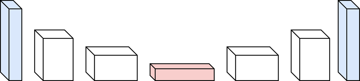
An autoencoder is a neural network trained to reconstruct its input from a compressed bottleneck. Trained only on normal data, it learns to reconstruct normal patterns well — and fails on anomalies.

Stacked autoencoder: input is compressed to a bottleneck latent code, then reconstructed. MSE loss between input and reconstruction drives training.

MSE Reconstruction Loss

$$\text{MSE Loss}: \quad l(x, y) = \frac{1}{N} \sum_{n} (x_n - y_n)^2$$ where $x$ is the original input and $y$ is the reconstruction. Anomaly detection: high loss = anomaly.

How Autoencoders Detect Anomalies

Train the autoencoder on only normal data. Minimize reconstruction error on normal patterns.
During testing, compare the reconstructed version with the original input.
If the reconstructed version differs greatly from the input (high MSE), the input is anomalous — the autoencoder cannot reconstruct something it never saw during training.

Denoising Autoencoders

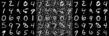
Denoising autoencoder: MNIST digits with noise added (left), fed through the encoder-decoder, producing clean reconstructions (right). Loss is computed against the original clean image.

A denoising autoencoder adds noise to the input before encoding, but computes the loss against the original clean image. This forces the network to learn robust representations of the underlying clean signal. During anomaly detection, the model improves on normal examples over training but produces high loss on unseen outliers.

Four Autoencoder Hyperparameters

Hyperparameter	Description
Code size	Number of nodes in the bottleneck layer; smaller = more compression
Number of layers	Depth of encoder and decoder
Nodes per layer	Decreases through encoder; increases symmetrically through decoder
Loss function	Typically MSE loss

8. Convolutional Autoencoders (CAEs)

State-of-the-art anomaly detection uses Convolutional Autoencoders — much better than fully-connected autoencoders for image/video data.

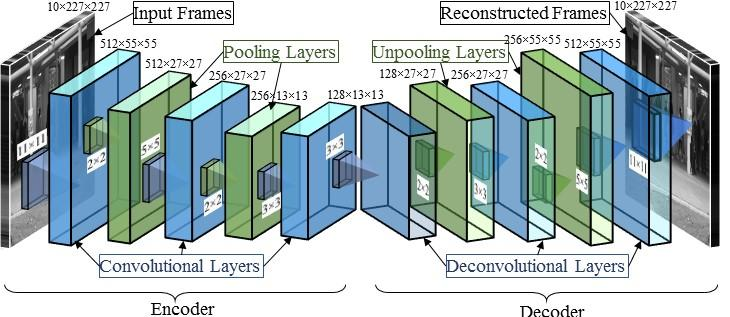
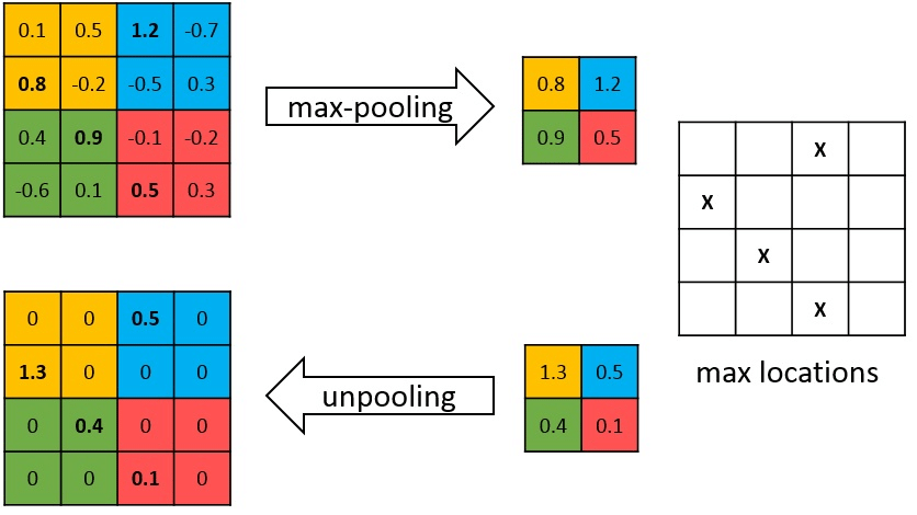
CAE architecture: convolutional + pooling encoder layers compress input (e.g., 10x227x227 frames) to a latent representation; deconvolutional + unpooling decoder layers reconstruct the original dimensions.

Pooling and Unpooling

Max-pooling (encoder): selects maximum per local region, reduces spatial size, stores max locations. Unpooling (decoder): places values back at stored max locations; zeros elsewhere.

Pooling vs unpooling, convolution vs deconvolution

Summary: pooling reduces spatial size; unpooling restores it using stored locations. Convolution extracts features (many-to-one); deconvolution reconstructs (one-to-many).

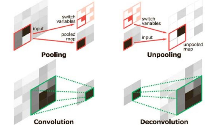
Transposed Convolution (Deconvolution)

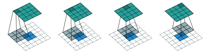
The deconvolution (transposed convolution) layer recovers spatial dimensions in the decoder:

Convolution: maps a larger input region to a smaller output (many-to-one). Reduces spatial dimensions.
Deconvolution: maps a smaller input to a larger output (one-to-many). Increases spatial dimensions.

Transposed convolution step-by-step: each input value multiplied by the kernel and stamped into a larger output region, with overlapping regions summed.

9. I3D Architecture

I3D (Inflated 3D ConvNet) is one of the most important architectures for video feature extraction. It converts successful 2D image classification networks into 3D video understanding networks through "inflation."

Inflation: From 2D to 3D Filters

Take a 2D convolutional filter of size $k \times k$ (pre-trained on ImageNet). Repeat its weights $N$ times along the temporal dimension to create a $k \times k \times N$ 3D filter. Divide all weights by $N$ to preserve activation magnitudes.

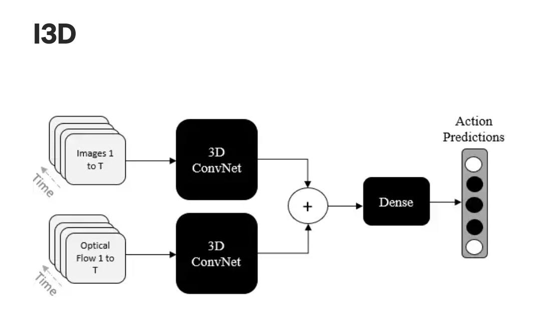
I3D two-stream architecture: RGB images and optical flow each processed by a 3D ConvNet independently, dense layers fuse predictions.

I3D Two-Stream Design

RGB stream: Processes raw video frames through 3D CNN to capture appearance + motion jointly.
Optical flow stream: Processes pre-computed optical flow fields through a separate 3D CNN to capture motion explicitly.
Fusion: Both stream predictions are combined for the final action classification.

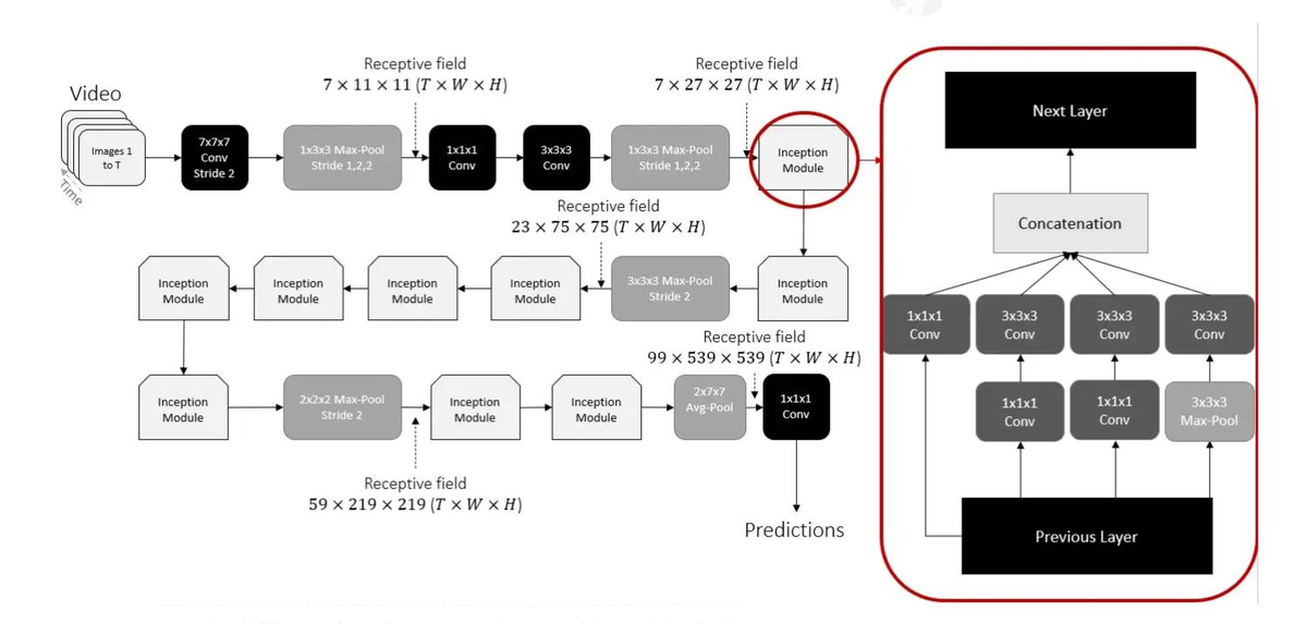
3D Inception Module

I3D uses Inception-style modules that allow the network to grow wider instead of deeper. Parallel branches with different filter sizes are concatenated, capturing features at multiple scales simultaneously:

I3D detailed architecture with inception modules

Detailed I3D architecture: series of 3D convolutions and pooling layers with growing receptive fields, punctuated by 3D inception modules. Receptive field shown at each stage ($T \times W \times H$).

Receptive Field in I3D

The receptive field (RF) is the region in the input contributing to one output feature. For 3D video CNNs, the RF has three dimensions: temporal $T$, width $W$, height $H$.

Asymmetric pooling strides

I3D uses pooling strides like (1,2,2) — subsampling spatial dimensions without subsampling time. This carefully controls how the temporal and spatial receptive fields grow. If the temporal RF grows too fast, it merges features from different objects across frames. If too slow, the network misses scene dynamics.

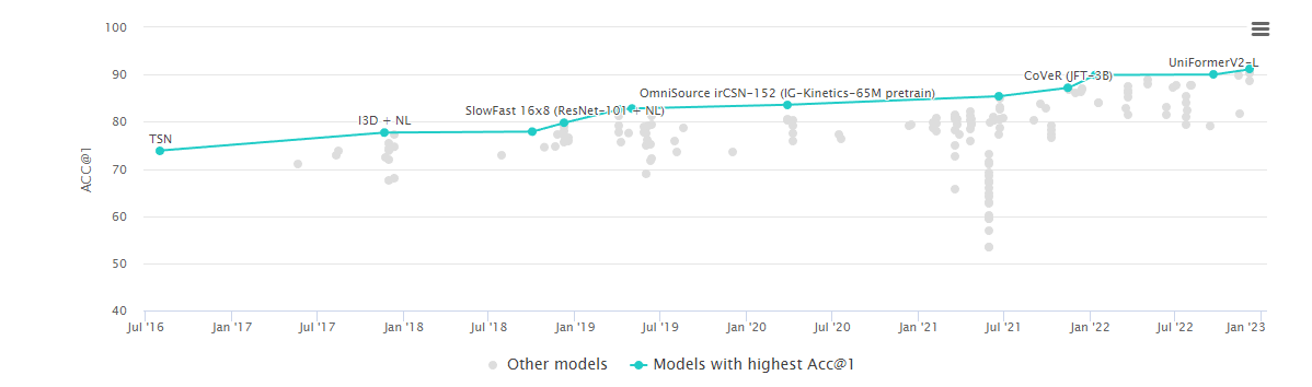
Kinetics Dataset Progress

Model	Year	Kinetics Top-1 Accuracy
TSN	Jul 2016	~73%
I3D + NL	Jan 2018	~78%
SlowFast 16x8 (ResNet-101 + NL)	Jan 2019	~80%
OmniSource irCSN-152	~2020	~84%
CoVeR (JFT-3B)	Jan 2022	~88%
UniFormerV2-L	Jan 2023	~90%

Progress on Kinetics dataset: top-1 accuracy improved from ~73% (TSN, 2016) to ~90% (UniFormerV2-L, 2023) over 7 years.

10. Multiple Instance Learning (MIL) for Anomaly Detection

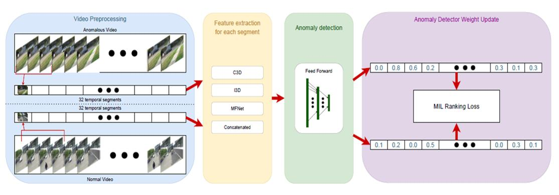
MIL is a weakly supervised learning paradigm suited for video anomaly detection where only video-level labels are available (not frame-level).

MIL Key Concept

A bag is a video; an instance is a temporal segment of that video.
A bag is labeled negative if ALL instances are negative (all segments are normal).
A bag is labeled positive if at least one instance is positive (at least one segment is anomalous).

MIL Pipeline for UCF Crime Dataset

The UCF Crime dataset contains 1,900 videos, 128 hours total, 13 anomaly classes (Accident, Burglary, Fighting, Robbery, Shooting, etc.).

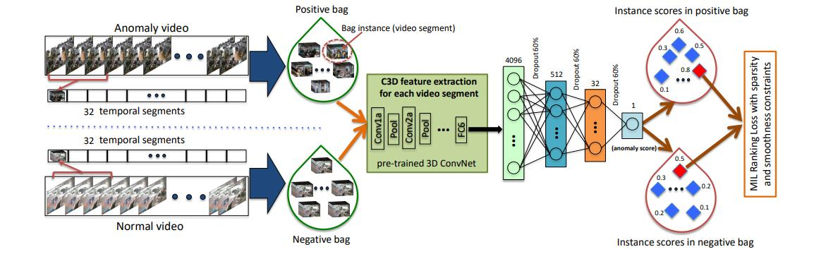
MIL pipeline: each video divided into 32 temporal segments (instances in a bag); C3D features extracted per segment; anomaly scores assigned; MIL ranking loss trained on score differences between positive and negative bags.

Divide each video into 32 temporal segments (bag instances).
Extract features from each segment using a pre-trained 3D ConvNet (C3D/I3D), producing 4096-dim feature vectors.
A fully connected network assigns an anomaly score to each segment.
Train with a MIL ranking loss: the maximum score in the positive bag must exceed the maximum score in the negative bag.

Throwing action detection: multiple backbone feature extractors (C3D, I3D, MFNet) combined with MIL ranking loss to detect throwing events in traffic surveillance.

11. SlowFast Architecture

The SlowFast network is designed based on the observation that video frames typically contain both static areas (which do not change) and dynamic areas (which indicate important ongoing events). Two parallel pathways handle each type:

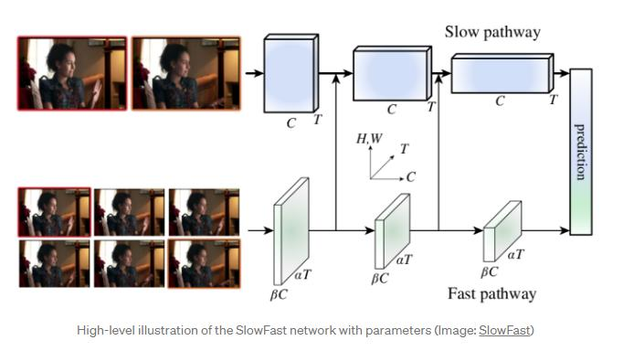
SlowFast network: slow pathway (low frame rate, high channel count) captures spatial semantics; fast pathway (high frame rate, low channel count) captures motion. Lateral connections fuse pathways.

Pathway	Frame Rate	Channel Capacity	Purpose
Slow pathway	Low (few frames)	High ($C$ channels)	Capture spatial semantics, appearance, scene context
Fast pathway	High (many frames)	Low ($\beta C$, $\beta \ll 1$)	Capture motion at fine temporal resolution

Design rationale

Fine temporal processing does not need rich spatial detail. The fast pathway can be lightweight (few channels) because it only needs to capture motion patterns, not detailed appearance. Lateral connections fuse motion information from the fast pathway into the rich spatial representation of the slow pathway.

Density-Guided Label Smoothing

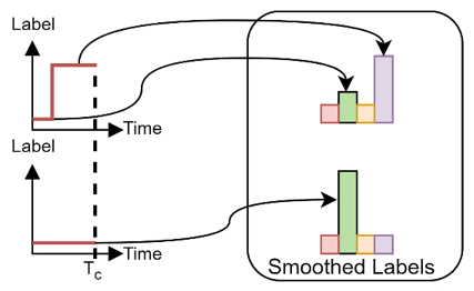
Video segments at action boundaries contain multiple action types. Assigning the dominant class as a hard label gives misleading gradient signals. Density-guided label smoothing assigns target probabilities proportional to how densely each class appears in the segment:

Example: a segment that is 70% "texting" and 30% "phone call" gets smoothed label [0.7, 0.3] rather than hard label [1, 0]. This is critical for strict temporal localization (the distracted driver task requires ±1 second accuracy).

Density-guided label smoothing: multi-label and single-label segments mapped to smoothed probability distributions for more accurate boundary localization.

12. Crowd Behaviour Analysis

Crowd Density Estimation: Multi-Column CNN

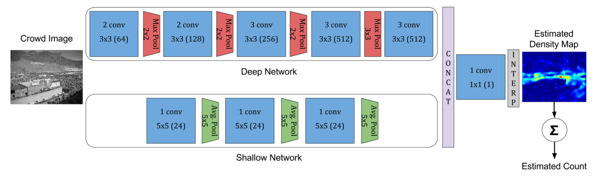
This architecture combines deep and shallow CNNs to generate a crowd density map:

Deep network path: VGG-like (3×3 convolutions, max pooling) — recognizes high-level semantic cues (heads, torsos) for nearby subjects.
Shallow network path: Wide filters (5×5, average pooling) — detects low-level features (blobs, edges) for distant subjects that appear small.

Both paths are concatenated, passed through a 1×1 convolution, and interpolated to produce the density map. The estimated count = sum of all density map pixel values.

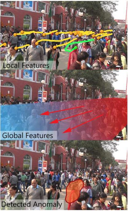
Multi-column CNN for crowd density estimation: deep network for nearby subjects and shallow network for distant subjects, combined to produce a density map; count = sum of density values.

Crowd Anomaly Detection: Kalman + K-Means

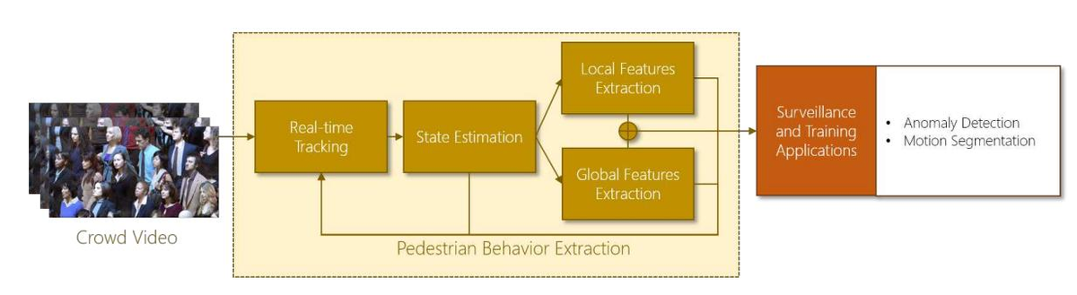
Crowd anomaly detection pipeline: real-time tracking, state estimation (Kalman filter), local feature extraction, global feature via k-means, anomaly declaration by distance threshold.

Real-time tracking: Detect and track each pedestrian in the scene.
State estimation (Kalman filter): Estimate each person's position and velocity over time.
Local features: For each person, concatenate their state (position + velocity) over a temporal window.
Global feature (k-means): Apply k-means to all local features. The largest cluster = the global (dominant normal) motion pattern.
Anomaly detection: If a person's local feature is too far (by some distance metric) from the global feature, declare an anomaly (e.g., walking against the crowd flow).

Crowd anomaly detection: local features (individual motion arrows), global features (dominant flow direction), and detected anomalies (pedestrians deviating from dominant pattern).

Interactive: I3D and Anomaly Detection Walkthrough

Flashcards

← 12. Data Analysis